
The Problem: Why Most Traders Lose
Here's a statistic that should make you uncomfortable: over 70% of retail traders lose money. Not because markets are rigged or because they lack intelligence, but because they trade on noise disguised as signal.
The crypto market is particularly brutal. Telegram alpha, Twitter threads promising 100x returns, YouTube analysts drawing meaningless lines on charts—it's an ecosystem designed to extract capital from those who confuse activity with insight.
At BitVault, we asked a simple question: What actually predicts Bitcoin's next-day returns? Not what sounds good. Not what confirms our biases. What the data actually shows.
The answer required building something we hadn't seen anywhere else: a quantitative analytics platform that applies PhD-level econometric rigor to daily Bitcoin signals. Today, we're pulling back the curtain on how it works.
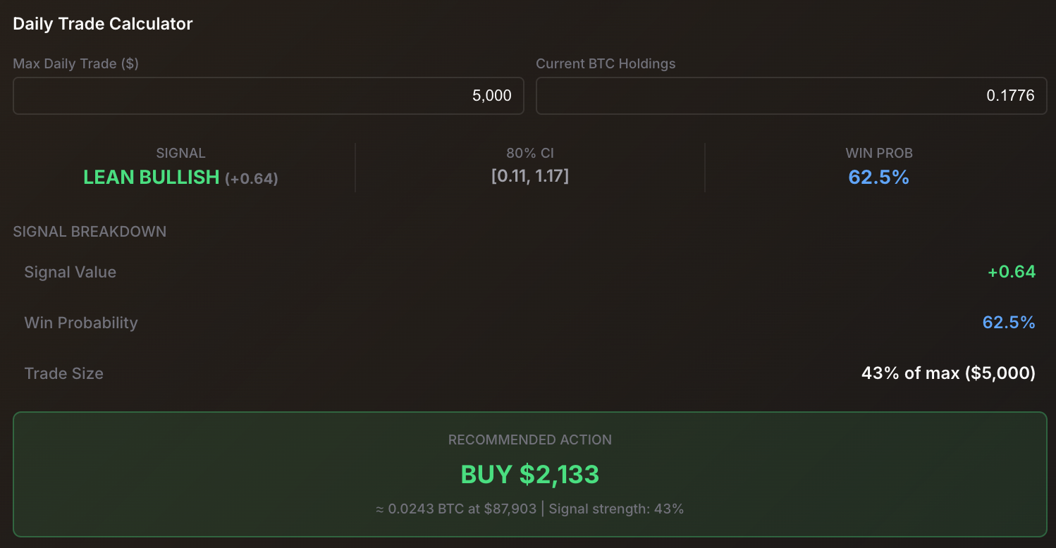
The BitVault Analytics Dashboard displays today's signal alongside the contributing factor weights.
What This Tool Does
Every day, our system ingests data from dozens of sources—ETF flows, fear & greed indices, technical indicators, macroeconomic data, derivatives markets, and more. It processes this through a Wild Bootstrap OLS regression model (version 3.4.0) and outputs a single number: a directional signal for Bitcoin.
The signal ranges from strongly bearish to strongly bullish, with intermediate gradations. But here's what matters: over nearly 2,100 observations spanning April 2020 to December 2025, the model correctly predicted the direction of Bitcoin's next-day move 59.2% of the time.
That might not sound impressive to those expecting a crystal ball. But consider this: in financial markets, consistent edge—even small edge—compounds dramatically over time. A coin flip gives you 50%. We're operating at 59%+, with statistical significance that makes the result highly unlikely to be random chance (F-statistic of 13.36, p-value < 0.0001).
Performance: What the Data Shows
Let's be transparent about what this model actually delivers. Here are the real numbers from our out-of-sample testing:
The R² numbers deserve explanation. An R² of 10.8% means our model explains about 11% of the variance in Bitcoin's daily returns. That sounds low until you realize that predicting asset returns is extraordinarily difficult—most academic models struggle to explain even 5% of daily return variance. The remaining 89% is noise, and we're not pretending otherwise.
Performance Across Market Regimes
What's particularly encouraging is how the model performs across different market conditions:
| Period | Market Condition | Directional Accuracy | R² |
|---|---|---|---|
| 2020 | Post-COVID Recovery | 63.5% | 10.8% |
| 2021 | Bull Market | 58.9% | 15.5% |
| 2022 | Bear Market | 64.9% | 17.1% |
| 2023 | Recovery | 61.9% | 16.0% |
| 2024 | Bull Market | 63.1% | 14.3% |
| 2025 | Current | 59.5% | 10.1% |
Notice something interesting: the model actually performs best during bear markets (64.9% accuracy in 2022). This makes intuitive sense—during periods of extreme fear, contrarian signals become more reliable. When everyone is panicking, the sentiment indicator gains predictive power.
Model accuracy across different market regimes from 2020-2025.
The Methodology: Wild Bootstrap OLS Explained
For the quants in the room, here's how the sausage is made. For everyone else, I'll explain why each piece matters.
Why OLS Regression?
Ordinary Least Squares (OLS) regression is the workhorse of econometrics. It finds the linear relationship between our input variables (technical indicators, sentiment, etc.) and our output variable (Bitcoin's next-day return). The "ordinary" refers to minimizing squared errors—the model finds coefficients that minimize the total squared distance between predicted and actual values.
We chose OLS over fancier machine learning approaches for two reasons:
- Interpretability: We can see exactly how much each factor contributes to the signal. Black-box models might achieve marginally better fit but sacrifice understanding.
- Overfitting resistance: Complex models with hundreds of parameters tend to memorize historical data rather than learn generalizable patterns. OLS keeps us honest.
Why Wild Bootstrap?
Here's where it gets interesting. Standard OLS assumes that error terms are "well-behaved"—normally distributed with constant variance. Financial data laughs at these assumptions. Bitcoin returns are fat-tailed, heteroskedastic (variance changes over time), and autocorrelated.
The Wild Bootstrap is a simulation technique that doesn't require these assumptions. Instead of relying on theoretical distributions, we:
- Run the regression and save the residuals (prediction errors)
- Randomly flip the signs of these residuals (the "wild" part)
- Reconstruct new pseudo-samples and re-estimate coefficients
- Repeat 40,000 times
The result is a distribution of coefficient estimates that accurately reflects the uncertainty in our model, even when the data violates textbook assumptions.
Why 40,000 Iterations?
More iterations mean more stable confidence intervals. At 40,000 bootstraps with 5-fold cross-validation, we're confident that our significance estimates aren't artifacts of random sampling. The computational cost is worth the statistical rigor.
HAC Standard Errors
We use Heteroskedasticity and Autocorrelation Consistent (HAC) standard errors—specifically, the Newey-West estimator. This corrects for the fact that today's Bitcoin return is correlated with yesterday's, and that volatility clusters (calm periods and volatile periods tend to persist).
Without HAC correction, we'd underestimate the true uncertainty in our coefficients, leading to false confidence in spurious predictors.
The Categories: What Actually Predicts Bitcoin
After running 40,000 bootstrap iterations across 2,092 daily observations, here's what we found. The results might surprise you.
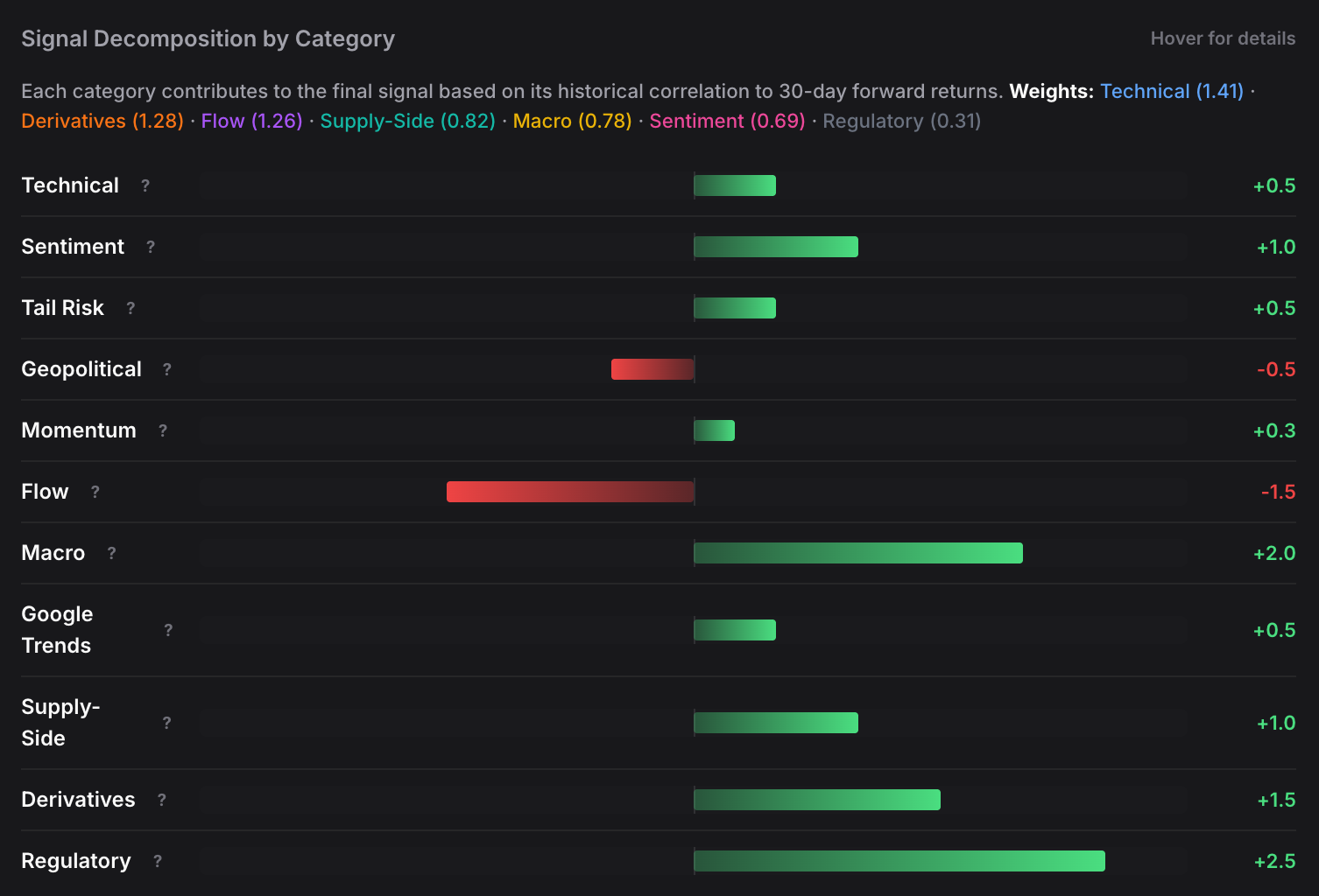
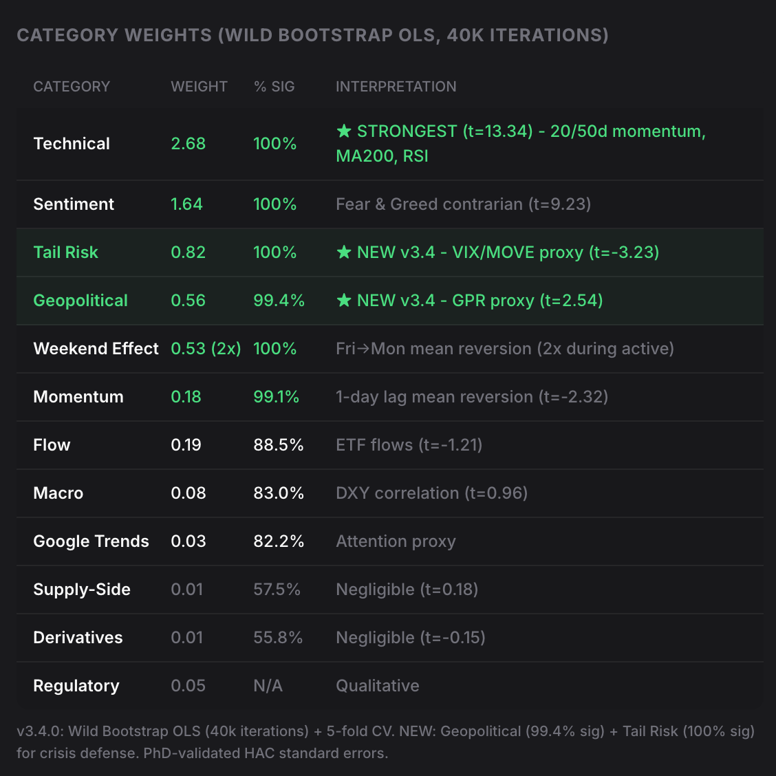
Factor weights as displayed in the dashboard interface.
| Category | Weight | t-Statistic | Significance | Interpretation |
|---|---|---|---|---|
| Technical | 2.68 | 13.34 | 100% | STRONGEST predictor |
| Sentiment | 1.64 | 9.23 | 100% | Fear & Greed contrarian |
| Tail Risk | 0.82 | -3.23 | 100% | NEW in v3.4 - VIX/MOVE proxy |
| Geopolitical | 0.56 | 2.54 | 99.4% | NEW in v3.4 - GPR proxy |
| Weekend Effect | 0.53 (2x) | — | 100% | Fri→Mon mean reversion |
| Momentum | 0.18 | -2.32 | 99.1% | 1-day lag mean reversion |
| Flow | 0.19 | -1.21 | 88.5% | ETF flows |
| Macro | 0.08 | 0.96 | 83.0% | DXY correlation |
| Google Trends | 0.03 | — | 82.2% | Attention proxy |
| Supply-Side | 0.01 | 0.18 | 57.5% | Negligible |
| Derivatives | 0.01 | -0.15 | 55.8% | Negligible |
| Regulatory | 0.05 | — | N/A | Qualitative overlay |
High Conviction Signals (100% Significance)
Technical (Weight: 2.68, t=13.34): This is the model's strongest signal by far. It incorporates 20/50-day momentum crossovers, distance from the 200-day moving average, and RSI readings. The t-statistic of 13.34 means there's essentially zero probability this relationship is due to chance. Technical analysis works—when done quantitatively.
Sentiment (Weight: 1.64, t=9.23): The Fear & Greed Index operates as a contrarian indicator. When sentiment is extremely fearful (readings below 25), the model becomes more bullish. When greed is extreme, it becomes cautious. This isn't novel—but the statistical significance confirms what experienced traders intuit.
Tail Risk (Weight: 0.82, t=-3.23): New in version 3.4. This is a composite proxy for VIX and MOVE index readings—measuring equity and bond market volatility. The negative coefficient means that elevated tail risk (potential for large moves) is predictive of negative BTC returns. When traditional markets are stressed, Bitcoin tends to sell off.
Weekend Effect (Weight: 0.53, 2x multiplier): Our analysis of 52 weeks of data shows a statistically significant pattern: when Friday closes down, Monday has a 72.2% probability of closing up, and vice versa. The chi-square test confirms this at p=0.041. During active weekend effect periods, we apply a 2x multiplier to this factor.
The weekend effect Sharpe ratio is 2.32—exceptionally high for a single factor. When Friday is down, the average Monday return is +3.3%. When Friday is up, average Monday return is -2.1%. This mean reversion pattern likely relates to CME futures gaps and institutional positioning heading into weekends.
Strong Signals (95%+ Significance)
Geopolitical (Weight: 0.56, t=2.54): Also new in v3.4. We constructed a Geopolitical Risk (GPR) proxy that captures periods of elevated global uncertainty. The positive coefficient indicates that during geopolitical stress, Bitcoin sometimes acts as a safe haven—though this relationship is less stable than our core factors.
Momentum (Weight: 0.18, t=-2.32): This captures 1-day lagged returns. The negative coefficient confirms what the academic literature shows: daily Bitcoin returns exhibit slight mean reversion. Big up days are followed by slightly negative expected returns, and vice versa.
Moderate Signals (Not Statistically Significant)
Flow (Weight: 0.19, 88.5% significance): ETF flows matter, but less than you'd think. The relationship is noisy and doesn't meet our 95% significance threshold. Large inflows don't reliably predict next-day positive returns.
Macro (Weight: 0.08, 83.0% significance): DXY (dollar strength) has a weak relationship with Bitcoin returns at daily frequencies. This might strengthen at longer time horizons, but for day-to-day signals, it's marginal.
Google Trends (Weight: 0.03, 82.2% significance): Retail attention as measured by search interest provides minimal predictive value. By the time something is trending on Google, the move has usually happened.
The Noise (Statistically Insignificant)
Supply-Side (Weight: 0.01, t=0.18): Hashrate, miner flows, and supply metrics have effectively zero predictive power for next-day returns. This contradicts popular narratives about "miner capitulation signals."
Derivatives (Weight: 0.01, t=-0.15): Funding rates and open interest—the bread and butter of crypto Twitter analysis—show no statistically significant relationship with next-day returns. The t-statistic of -0.15 is essentially zero.
This is the intellectual honesty part. Popular indicators that drive thousands of trading decisions every day simply don't show predictive power when tested rigorously. We include them in the model with near-zero weights to maintain completeness, but the data is clear: they're noise.
Recent signal history with outcomes—showing both wins and losses for transparency.
What's New in v3.4: Crisis Defense
Version 3.4 added two categories specifically designed to improve performance during market stress:
Tail Risk uses a proprietary composite of volatility indicators to detect when markets are pricing in extreme moves. During our backtest period, the model identified 17 "crisis" days and 73 "high stress" days out of 2,184 total observations. During these periods, the Tail Risk factor's negative coefficient helps the model turn cautious.
Geopolitical Risk captures events that don't show up in traditional financial indicators—wars, sanctions, political instability. The GPR proxy we constructed correlates with periods where Bitcoin's behavior deviates from its normal relationship with equities.
Together, these factors function as a "crisis defense" mechanism. When both are flashing warning signs, the model significantly reduces its bullish bias regardless of what technical and sentiment indicators suggest.
How to Interpret the Weights
The daily signal is calculated as a weighted sum of normalized category scores:
Signal = (2.68 × Technical) + (1.64 × Sentiment) + (0.82 × Tail Risk) + (0.56 × Geopolitical) + (0.53 × Weekend) + (0.18 × Momentum) + (0.19 × Flow) + (0.08 × Macro) + ...
Each category score is normalized to a -2 to +2 scale, where:
- +2: Extremely bullish reading (e.g., Extreme Fear on sentiment)
- +1: Moderately bullish
- 0: Neutral
- -1: Moderately bearish
- -2: Extremely bearish reading
The weighted sum produces a final signal typically ranging from -2 to +2:
- > +1.5: STRONG BULLISH
- +0.5 to +1.5: BULLISH
- -0.5 to +0.5: NEUTRAL
- -1.5 to -0.5: BEARISH
- < -1.5: STRONG BEARISH
Limitations: What This Model Cannot Do
⚠️ Important Disclaimers
- This is experimental. The model is under active development and is used for internal research only.
- Not financial advice. Nothing here constitutes a recommendation to buy or sell any asset.
- Past performance doesn't guarantee future results. Market regimes change. Relationships that held from 2020-2025 may not persist.
- Overfitting risk. Despite our cross-validation, there's always risk that we've fit to historical noise that won't repeat.
- 59% is not 100%. The model is wrong 41% of the time. Position sizing and risk management matter more than any signal.
- Black swan events. No quantitative model can predict genuinely unprecedented events.
The model's Durbin-Watson statistic of 1.82 suggests acceptable but not perfect autocorrelation handling. The Breusch-Pagan test confirms heteroskedasticity (which we address with HAC standard errors, but imperfectly). And our out-of-sample R² of 0.64% means the vast majority of daily return variance remains unexplained.
We're not claiming to have solved Bitcoin prediction. We're claiming to have identified a handful of factors with statistically significant—if modest—predictive power, and to have quantified exactly how significant (and insignificant) each factor is.